Assignment 4: LeNet, Embeddings & Visualizing Hidden Spaces

In this assignment, you will reimplement the classic LeNet architecture, one of the first CNNs. Additionally, you will get to know a TensorBoard tool that helps with visualizing high-dimensional spaces such as the hidden activations of neural networks.

LeNet

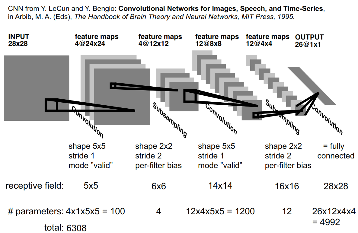
Implement LeNet based on this visual description. Note that “subsampling” is just average pooling (with stride 2), and of course you will need 10 output units instead of 26.

Embeddings in TensorBoard

In past assignments, we have seen that it is fairly simple to visualize the weights of a linear model and get an intuitive idea of their meaning. This is not so simple for deep models involving hidden layers. Convolutional layers can be visualized thanks to their known spatial structure, but no such structure exists for fully-connected layers. Luckily, TensorBoard comes with a tool to visualize such hidden spaces, which can give an impression of how well they represent the data and separate the different classes.

Setting up

This Tensorflow tutorial gives a short overview over what “embeddings” are (in our case, we can understand the layers of a network to compute embeddings of the input) as well as an overview over how to use TensorBoard’s built-in Embedding Projector. Unfortunately, this tutorial seems to have been cut in the recent update for unknown reasons and a lot of vital information is missing. A more complete version can be found here. The tutorial talks about tf.train.SummaryWriter at some point; replace this by tf.summary.FileWriter.

Try some visualizations for an MNIST model (MLP or CNN). You might want to proceed in the following steps:

• First, you need to make the variables you want to visualize available to the tf.train.Saver. Ignore anything regarding metadata for now. For example, you might want to visualize the activations of some hidden layer on (a part of) the test set. There’s a bit of a dilemma here: You will want to visualize activations of a trained network, but it seems like the Saver will only store variables defined before itself. Also, it is bad practice to add variables/ops to your graph after a session has launched. The following is a little annoying, but works (if you come up with a better way, feel free to share it!):
  • Define a tf.Variable with the appropriate shape to hold your embeddings (e.g. 1000x100 if you want to visualize a 100-dimensional hidden layer on 1000 elements of the test set). Fill it with whatever values; this will get overwritten.
  • Define a tf.assign op where you assign the hidden activation variable to the embedding variable.
  • Define the saver, train your network.
  • Run the assign op, feeding the appropriate input (e.g. the first 1000 elements of the test set) into the network input placeholder.
  • Save a checkpoint. Note: When saving multiple checkpoints, the most recent one will automatically be picked. Unfortunately, there seems to be no option to “scroll through” checkpoints at this time (e.g. to monitor how embeddings change through training). Now when you start TensorBoard, you should see a PROJECTOR tab. Here you can visualize any 2D tensor that was saved. Check that your variable is there and select it. If it’s something like the pre-output hidden layer of a properly trained network, you might already see some clustering in the visualizations, but it’s hard to see what’s going on because all points look the same. Let’s make them prettier.
• Supply a text file with label metadata. This can simply be a file with one digit per line, such as the label files supplied in the last assignment. Make sure you supply the correct labels: E.g. if you are visualizing the first 1000 elements of the test set, the metadata file should contain the first 1000 lines of the test set label file. You can either load this file via the Load data button in TensorBoard, or supply it directly in code as shown in the tutorial. You should then be able to color the dots by label. You can also replace the dots by labels via the button towards the top, next to where it says Points and Dimensions (3D labels mode).
• Finally, include a sprite image. Here we provide a function to generate such an image for a given subset of the data (there is also a simple function to extract part of a label file). This function hasn’t been tested much; please contact Jens in case of issues. The tutorial shows you how to include the image in TensorBoard.

Note: If using relative paths for the metadata/sprite image, this path should be relative to the saver path. I.e. if the saver saves to the logdir, the metadata paths should be relative to the logdir. The Tensorflow tutorial gives a different impression here.

Understanding the Visualizations

Now that we have some pretty images, you should consider what they actually mean. The n-dimensional data we supplied has automatically been reduced to two or three dimensions. You can choose between two methods for this: t-SNE or PCA. The Tensorflow tutorial has several links explaining these methods. Definitely read this one on t-SNE. Here is another one on PCA. Play around with the different options such as 2D/3D, t-SNE hyperparameters, or sphereizing the data or not (also note the effect on % explained variance for the PCA!).

Analyzing High-dimensional Spaces

Finally, use these visualization to gain some insights. For example, you could visualize the different layers of a network, from input to output, and observe how the data is progressively “disentangled”. You can also visualize convolutional layers by flattening the feature maps (i.e. reshaping them to 2D). It might be interesting to see how pooling changes the embeddings. Also, compare the pre-output layers of two models with differing performances – which one seems to have the “better” representation? Note that for linear models the pre-output layer is actually the raw input.

In general, do these visualizations make sense to you? Look out for some peculiarities of the MNIST data. Are some digits clustered more tightly than others? Look for outliers (with regard to a specific digit cluster) – do these generally look atypical? Which digits are “neighbors” in this space? You might want to concentrate on (non-sphereized) PCA for these qestions.